Signature Analysis Tutorial
This is a tutorial for SV signature analysis with Viola.
Requirements
If you are new to the Viola package, please refer to the Quick Start first. Quick Start explains basic usage of Vcf class, which shares a lot of methods with MultiBedpe class.
Installing “matplotlib” to your python environment is recommended.
In this tutorial, we use BEDPE files provided by ICGC Data Portal. Detailed instruction of data preparation is described below.
PCAWG data preparation
Create new directory named “resources” (Of cource you can name it otherwise) in your working directory and run
cd resources.Download
final_consensus_sv_bedpe_passonly.icgc.public.tgzandfinal_consensus_sv_bedpe_passonly.tcga.public.tgzto the “resources” directory.Run
tar zxvf final_consensus_sv_bedpe_passonly.icgc.public.tgzandtar zxvf final_consensus_sv_bedpe_passonly.icgc.public.tgzNow you’ve got the
icgc/directory and thetcga/directory.Create new directory named “pcawg” in the “resources” directory (This is also customizable).
Run
mv icgc/open/*.gz pcawgandmv tcga/open/*.gz pcawgRun
cd pcawg, then rungunzip *.gzNow you’ve got decompressed BEDPE files in the “pcawg” directory.
Other files preparation
Go back to the “resources” directory.
Visit here and prepare same directories and files (You’ve already prepared pcawg files by above instruction).
Decompress
replication_timing.bedgraph.gzby runninggunzip replication_timing.bedpe.gzGo back to your working directory and create new Jupyter Notebook file (You can also use the ipynb file uploaded on GitHub.).
Note
Example ipynb file is available on GitHub!
Warning
Due to the very large amount of data in PCAWG, the code described below will also take long time (around 50 min on Google Colab). If you want to try it in a shorter time, reduce the number of files in the directory.
Generate Matrix
Here, we explain how to generate SV feature matrix with custom SV class. In this tutorial, we are going to classify SV by:
Classify the SVs into DEL, DUP, INV, and TRA, and then subclassify them according to their size.
Common fragile sites
Replication timing
This can be achieved with only eight lines of code. The actual code is shown below.
import viola
pcawg_bedpe=viola.read_bedpe_multi('./resources/pcawg/', svtype_col_name='svclass' ,exclude_empty_cases=True)
bed_fragile = viola.read_bed('./resources/annotation/fragile_site.hg19.bed')
bedgraph_timing = viola.read_bed('./resources/annotation/replication_timing.bedgraph')
pcawg_bedpe.annotate_bed(bed=bed_fragile, annotation='fragile', how='flag')
pcawg_bedpe.annotate_bed(bed=bedgraph_timing, annotation='timing', how='value')
pcawg_bedpe.calculate_info('(${timingleft} + ${timingright}) / 2', 'timing')
feature_matrix = pcawg_bedpe.classify_manual_svtype(definitions='./resources/definitions/sv_class_definition.txt', return_data_frame=True)
Now let’s look at what each line means!
1. Importing Viola
import viola
2. Reading BEDPE files into viola.MultiBedpe object
pcawg_bedpe=viola.read_bedpe_multi('./resources/pcawg/', svtype_col_name='svclass', exclude_empty_cases=True)
This code reads all BEDPE files in the ./resources/pcawg directory into MultiBedpe class (See MultiBedpe).
Because the BEDPE files created by PCAWG have the svclass columns, we passed it to the svtype_col_name argument
Some BEDPE files did not have any SV records. This time we will exclude these by setting exclude_empty_cases=True.
3. Reading BED/BEDGRAPH files for annotation
bed_fragile = viola.read_bed('./resources/annotation/fragile_site.hg19.bed')
bed_timing = viola.read_bed('./resources/annotation/replication_timing.bedgraph')
Reading BED and BEDGRAPH files required for custom SV classification. At the moment we do not make a clear distinction between BED files and BEDGRAPH files. This is because only the first four columns of these files are used for annotation purposes in the first place.
fragile_site.hg19.bed is a BED file specifying the known common fragile site (CFS) regions.
replication_timing.bedgraph is a BEDGRAPH file which records the replication timing for each genome coordinate divided into bins.
These files were built according to the PCAWG paper.
4. Annotating SV
pcawg_bedpe.annotate_bed(bed=bed_fragile, annotation='fragile', how='flag')
pcawg_bedpe.annotate_bed(bed=bedgraph_timing, annotation='timing', how='value')
In this step, we annotate pcawg_bedpe with the Bed object we’ve just loaded.
After annotation, new INFO – ‘fragileleft’, ‘fragileright’, ‘timingleft’, and ‘timingright’ – will be added.
Because two breakends form a single SV, ‘left’ and ‘right’ suffix are added.
When how='flag', annotate True/False according wether each breakend is in the range in the Bed (4th column of the Bed is ignored).
When how='value', annotate the value of 4th column of Bed if the breakends hit.
5. Get Average values of Replication Timing
pcawg_bedpe.calculate_info('(${timingleft} + ${timingright}) / 2', 'timing')
To get representative values of replication timing for each SV breakpoints, we decided to take mean values of two breakends. This code adds new INFO named ‘timing’ by calculating mean values of ‘timingleft’ and ‘timingright’.
6. Classify SV and Generate Feature Matrix
feature_matrix = pcawg_bedpe.classify_manual_svtype(definitions='./resources/definitions/sv_class_definition.txt', return_data_frame=True)
Finally, we classified SV according to its type, size, fragile site, and replication timing. Classification criteria are written in sv_class_definition.txt. Syntax of this file is explained below.
If return_data_frame=True, counts of each custom SV class for each patients are returned as pandas.DataFrame.
Now we successfully obtained feature matrix with custom SV classification!
Definition File Syntax
name 'At fragile site DEL'
0 fragileleft == True
1 fragileright == True
2 svtype == DEL
logic (0 | 1) & 2

name 'At fragile site DUP'
0 fragileleft == True
1 fragileright == True
2 svtype == DUP
logic (0 | 1) & 2

name '<50 kb early DEL'
0 svlen > -50000
1 timing > 66.65
2 svtype == DEL
logic 0 & 1 & 2

name '<50 kb mid DEL'
0 svlen > -50000
1 timing > 33.35
2 svtype == DEL
logic 0 & 1 & 2

name '<50 kb late DEL'
0 svlen > -50000
1 svtype == DEL
logic 0 & 1
This is an example of definition file of custom SV classification.
Each SV class is defined by a syntax like the following:
name '<SV class name>'
0 <condition>
1 <condition>
2 <condition>
...
logic <set operation>
The syntax of <condition> is the same as query passed to Vcf.filter method (See Quick Start).
The numbers written in the left of each <condition> can be omitted.
Use numbers correspoinding to each <condition> for the <set operation>
Note
The order of the SV class definition is very important. The classify_manual_svtype method reads the definition file in order from the top, so that the SV class definitions written higher up in the file take precedence. Thus, in above example, Deletions that both satisfy ‘At fragile site DEL’ and ‘<50 kb early DEL’ criteria, they are classified as ‘At fragile site DEL’, not ‘<50 kb early DEL’.
Signature Extraction
Viola offers the function, viola.SV_signature_extractor which performs non-negative matrix factorization (NMF) and cluster stability evaluation at the same time.
Before diving into the details of viola.SV_signature_extractor, let’s look at an example usage.
feature_matrix.drop('others', axis=1, inplace=True) # remove "others" column

result_silhouette, result_metrics, exposure_matrix, signature_matrix = viola.SV_signature_extractor(
feature_matrix, n_iter=10, name='testRun', n_components=2, init='nndsvda', solver='mu', beta_loss='kullback-leibler', max_iter=10000, random_state=1
)

######## STDOUT ########
# testRun: finished NMF
# testRun: finished kmeans clustering
# testRun: finished all steps
# Silhouette Score: 0.9997561882187715, kullback-leibler: 98901.64510245458
#
# ==================
viola.SV_signature_extractor outputs four returns. We will explain them one by one.
- result_silhouette:
This is the score that indicates the stability (reproducibility) of the SV signature. Detailed explanations are given below.
- result_metrics:
An error between the original matrix and the product of the factored matrice.
- exposure_matrix:
An exposure matrix with (n_samples × n_signatures).
- signature_matrix:
A result SV signature matrix with (n_signatures × n_features). Here,
n_featuresmeans “the number of custom SV class”
Viola employs NMF class of Scikit Learn for signature extraction. So, viola.SV_signature_extractor receives completely the same arguments of `sklearn-decomposition.NMF<NMF class of Scikit Learn>`_ except the first three, which are the original arguments of Viola.
Here are the explanations for Viola original arguments of viola.SV_signature_extractor
- X:
A (n_sample, n_features) shaped ndarray or DataFrame. Each column represents each SV class.
- n_iter:
Number of bootstrap resampling from X. The higher this number, the more reliable the result.
- name:
Name of this run.
Hyperparameter Tuning
For signature analysis, hyperparameters such as the number of signatures and the loss function need to be determined.
Here is an example of the hyperparameter tuning.
ls_silhouette = []
ls_metrics = []
ls_exposure = []
ls_signature = []
for num_signature in range(2, 15):
   print('Number of Signature: ' + str(num_signature))
   result_silhouette, result_metrics, exposure_matrix, signature_matrix = viola.SV_signature_extractor(
      feature_matrix,
      n_iter=10,
      name='testRun',
      n_components=num_signature,
      init='nndsvda',
      solver='mu',
      beta_loss='kullback-leibler',
      max_iter=10000,
      random_state=1
   )

 ls_silhouette.append(result_silhouette)
 ls_metrics.append(result_metrics)
 ls_exposure.append(exposure_matrix)
 ls_signature.append(signature_matrix)

######## STDOUT ########
# Number of Signature: 2
# testRun: finished NMF
# testRun: finished kmeans clustering
# testRun: finished all steps
# Silhouette Score: 0.9995314504820613, kullback-leibler: 98898.80582214911

# ==================

# Number of Signature: 3
# testRun: finished NMF
# testRun: finished kmeans clustering
# testRun: finished all steps
# Silhouette Score: 0.9996664503915801, kullback-leibler: 75815.89695274398

# ==================

# Number of Signature: 4
# testRun: finished NMF
# testRun: finished kmeans clustering
# testRun: finished all steps
# Silhouette Score: 0.9219878473698799, kullback-leibler: 65871.09184405269

# ==================

# ...
In order to determine the number of signatures based on the balance between the silhouette score and the Kullback-Leibler distance, let’s visualise the data.
%matplotlib inline
import matplotlib.pyplot as plt

fig = plt.figure()
ax1 = fig.add_subplot(111)

x = [i+2 for i in range(len(ls_silhouette))]

ln1 = ax1.plot(x, ls_silhouette,'C0', label="silhouette score")
ax2 = ax1.twinx()
ln2 = ax2.plot(x, ls_metrics,'C1', label="KL Divergence")
h1, l1 = ax1.get_legend_handles_labels()
h2, l2 = ax2.get_legend_handles_labels()
ax1.legend(h1+h2, l1+l2, loc='upper right')
ax1.set_title('Silhouette Score vs KL Divergence')
ax1.xaxis.set_major_locator(plt.MultipleLocator(1))
ax1.xaxis.grid(True)
ax1.set_xlabel('Number of Signatures')
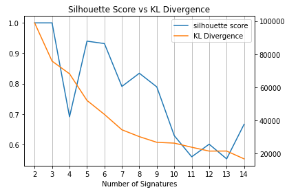
Now we can have a discussion that the number of signatures should be around 7-9.
The biological consideration is needed to determine the most appropreate number (Not the main topic here).
What does this function do?
Editing in progress…